CS184 Final Project

Anthony Ebiner, Shruteek Mairal, Srisai Nachuri, Maddy Chen

Abstract

A very common rendering task in animation is an accurate rendering of explosions in a wide variety of applications such as cinematography, video games, and physics simulations. For our final project, we built a GPU accelerated explosion simulation, simulating hundreds of thousands of particles modeled after realistic physics. These animations were built upon 3 modules: a Physical System, Visualizer, and Raytracer. The Physical System combined both particle and fluid physics by modeling the interactions between combusting fluid particles and corresponding temperature and velocity changes in a particle’s surrounding fluid cell. In turn, the fluid system would dictate the motion of fluid, drag force on particles, and energy transfer between different cells and particles. Utilizing the fluid system was intended to help the particles move in a non-uniform, physically accurate manner that more closely resembled abstract shapes of fire and explosions. After each timestep, the particles were passed into a Visualizer system, which converted particles into primitives, including taking into account particle radius and temperature to convert to RGB values for a bidirectional scattering distribution function. Lastly, these primitives were passed into the Raytracer module, which would render the frames that we stitched together to create the animations. The raytracer was run with a GPU and was heavily optimized through CUDA-acceleration, function optimization, and compatibility integration with various file types in order to support rendering massive numbers of primitives quickly.

Please see an overview of this project in our final project video.

Technical approach

Our animations relied on 3 modules to produce our final output: Raytracer, Physics, and Visualizer systems.

Module 1: CUDA-Accelerated GPU Raytracer

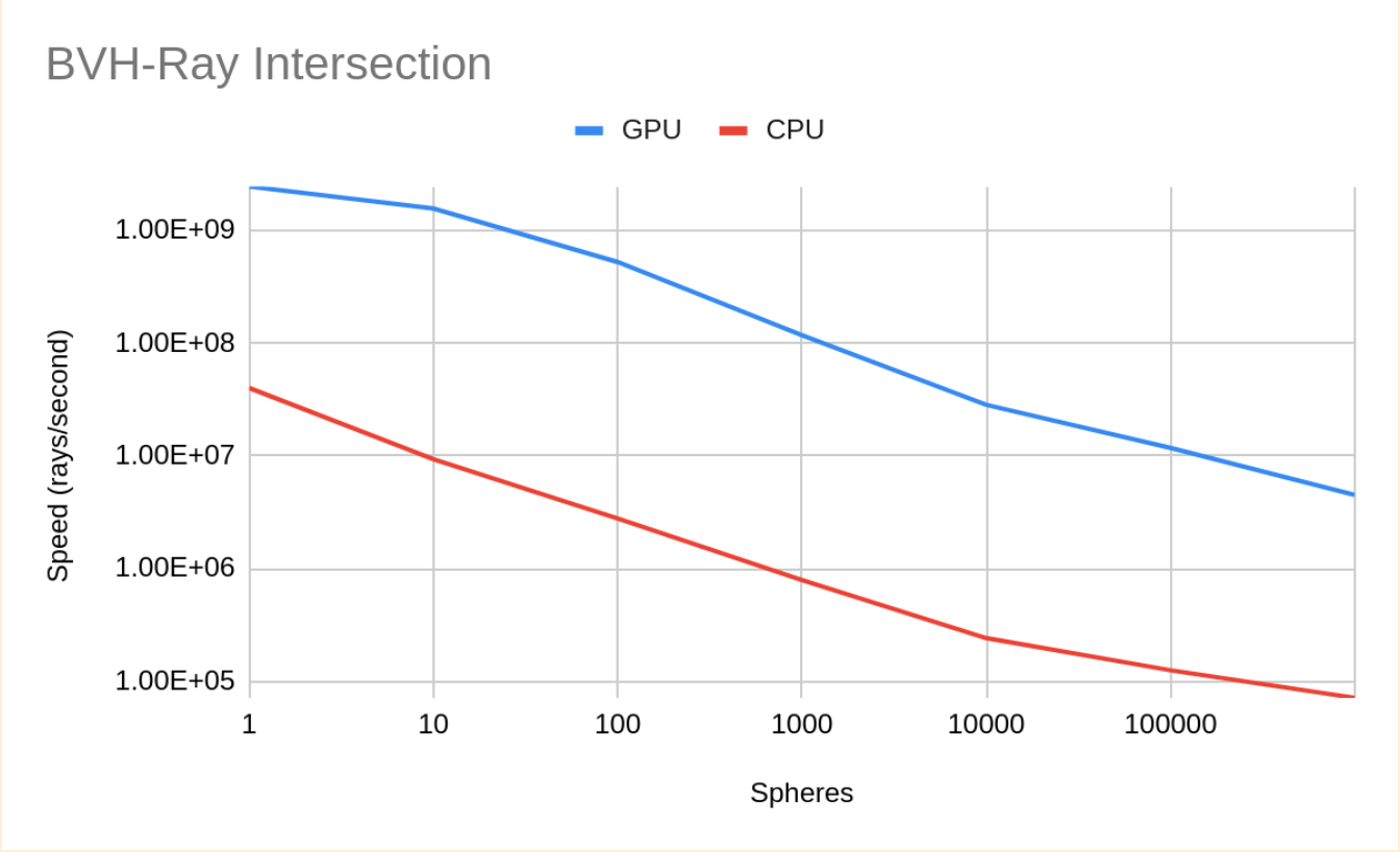
In order to render hundreds of thousands of particles, our raytracer needed to be heavily optimized so that frames could render in a reasonable time period. Building off of project 3, the code was heavily modified in order to support running the raytracer on a GPU via CUDA.

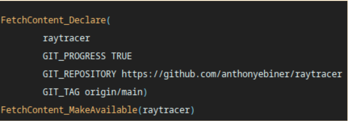
Several optimizations enabled lighting-fast rendering. These included writing a spatially contiguous BVH implementation (with BVH nodes using only 32 bytes of code), using floats instead of doubles, speeding up intersection tests, writing a fast XORShift random implementation, and using iterative ray bouncing instead of recursive ray bouncing. Converting the code to utilize the GPU’s CUDA cores was a significant undertaking, and required refactoring nearly all of the codebase. Additionally, since not all team members had access to the GPU, the raytracer was modified to be able to detect if the computer was a CUDA capable device, and to fall back to CPU rendering if it was not. This enabled all team members to test the rendering of the physics and visualizer systems regardless. The raytracer was also written as a header-only library, which allowed it to be easily imported into the other modules using the FetchContent dependency manager. To generate a larger library of images, the raytracer was also modified to be able to parse and load .OBJ and .MTL files, for more options of triangle meshes and materials. Overall, our accelerated implementation ended up being between 20 and 60 times faster than the previous version, which proved to be vital for rendering the explosions to come.

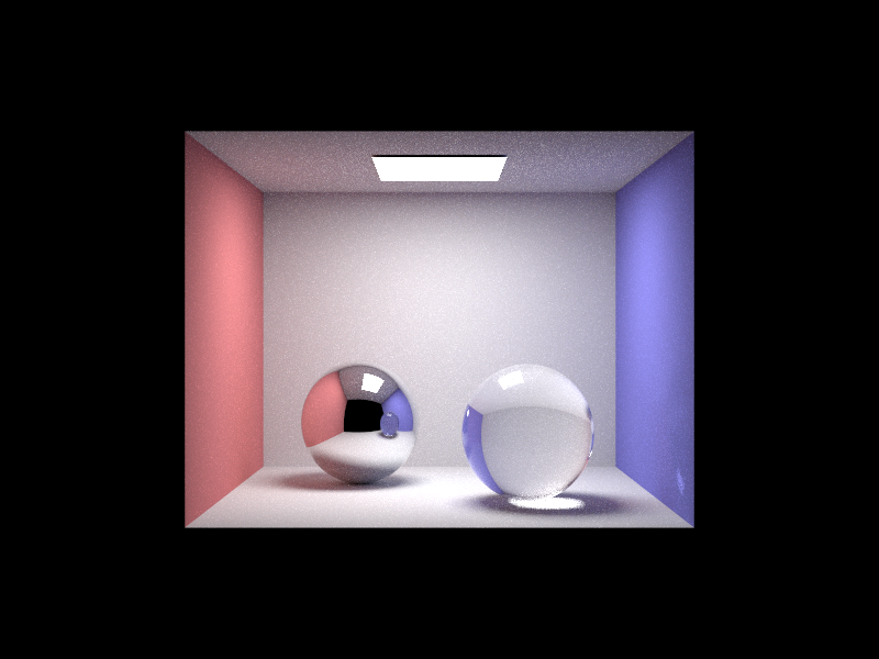
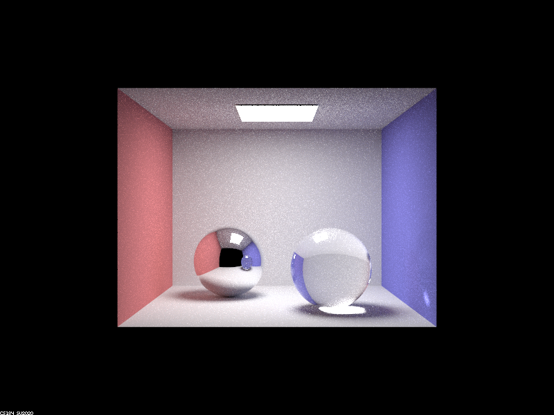
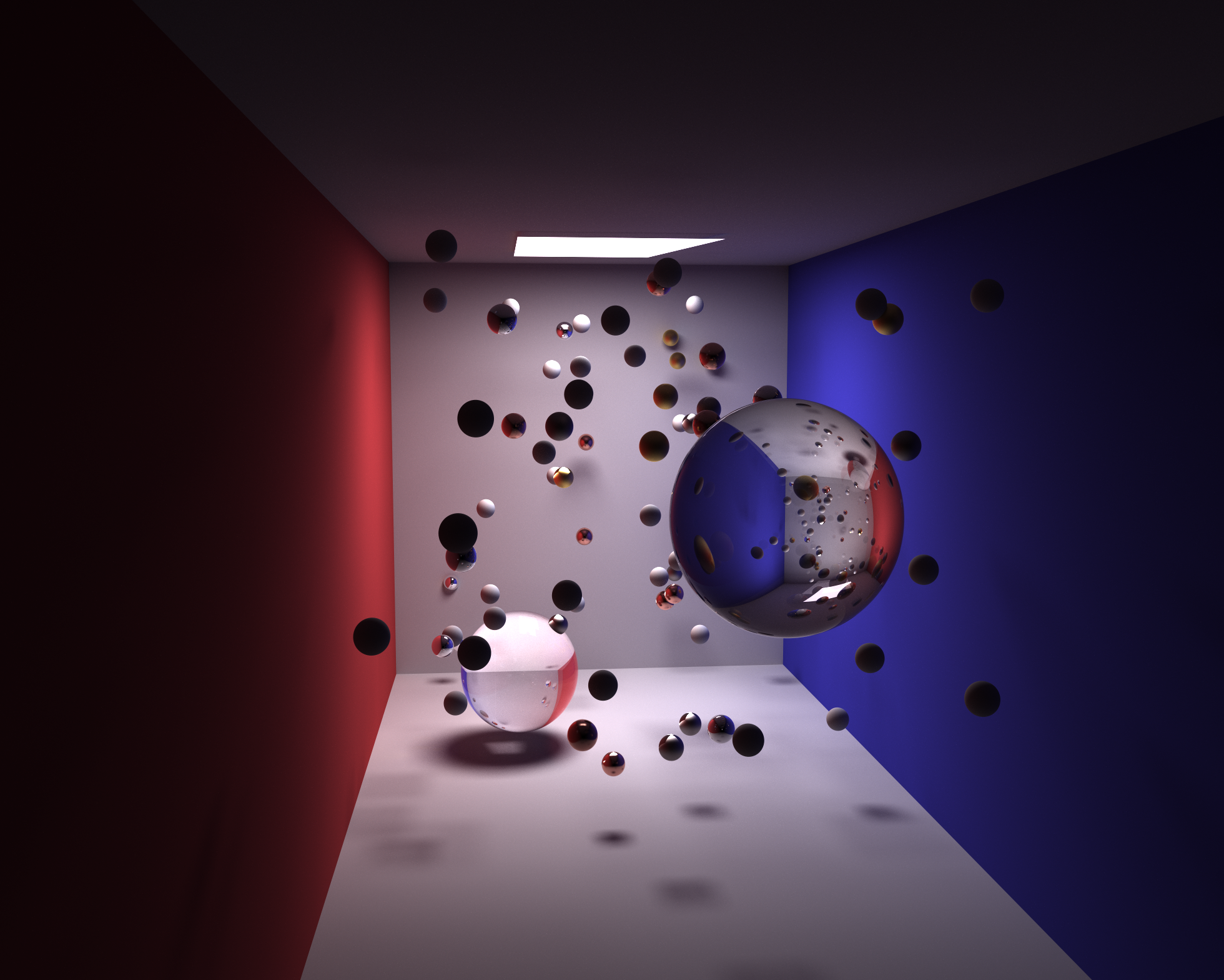
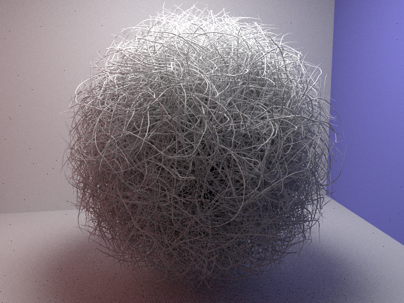
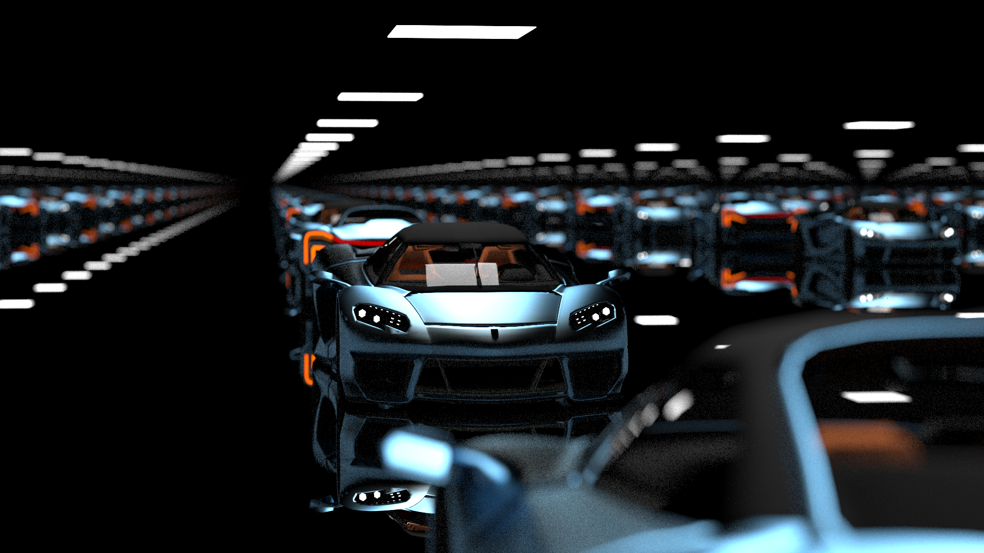
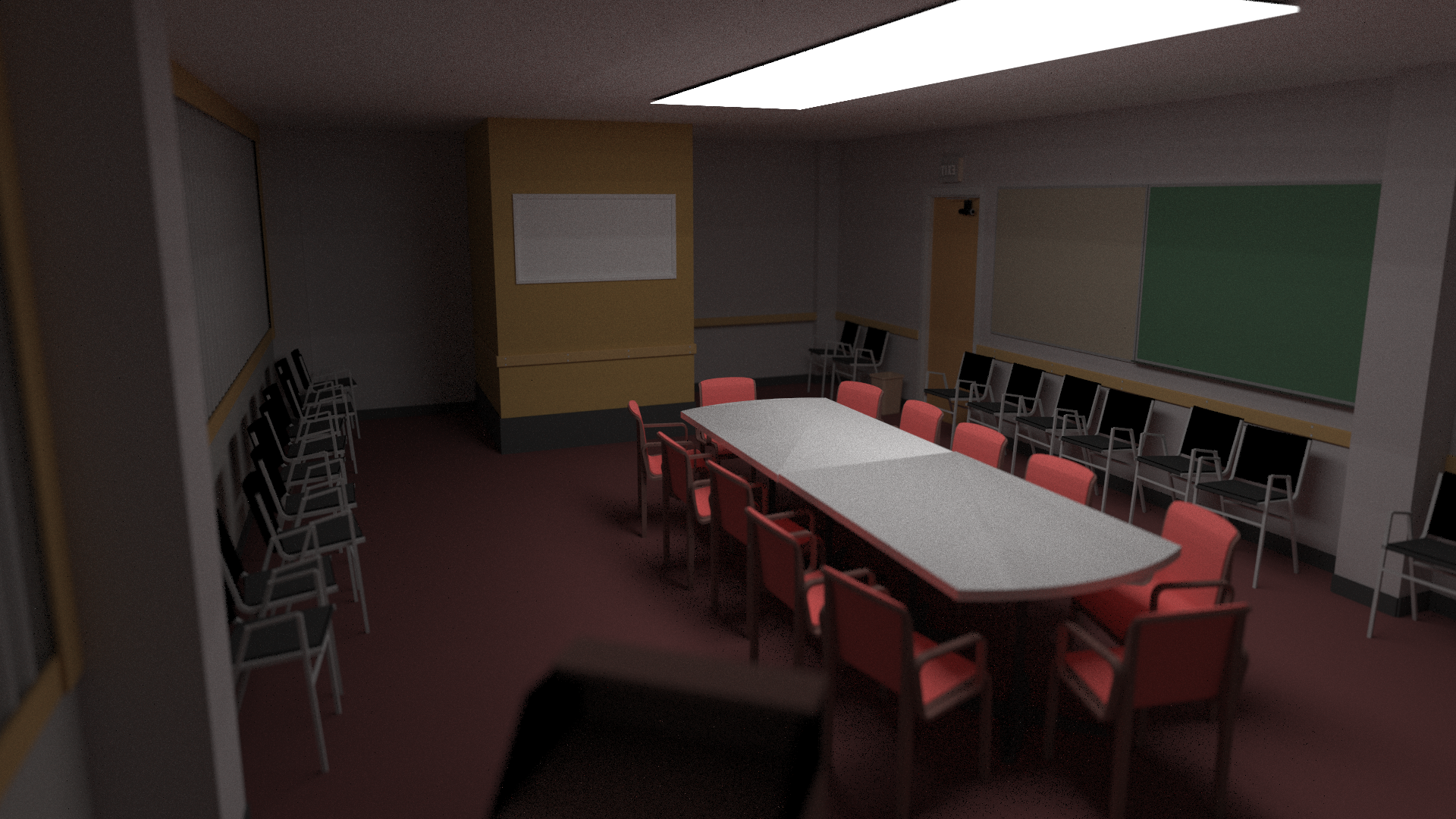
Renderings from the CUDA-accelerated raytracing, yielding a ~4000% speedup!!:

1k pixel samples, 4 light samples, 7 depth:

Accelerated Implementation

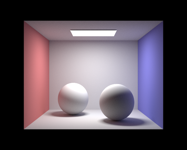
Project 3 Implementation

256 pixel samples, 4 light samples, 7 depth:

Module 2: Physics of Explosions

The second module handled all of the physics for our animations. Our model was primarily based on Animating Suspended Particle Explosions by Feldman, O’Brien, & Arikan, which uses a physical system for suspended particle explosions supported by an incompressible, inviscid fluid model to better account for the motions of particles. The fluid system also derived heavily from Jos Stam’s 1999 Stable Fluids paper as well as Fedkiw et al.’s 2001 Visual Simulation of Smoke paper, with Navier-Stokes-simplifying assumptions including incompressibility, inviscid flow, continuity equation deviation, and force assumptions including vorticity confinement, thermal buoyancy, and drag force. The particle system was based primarily on the Feldman et al. paper due to its novel usage of both particle and fluid systems to simulate explosions, which was our main goal. Its particles interacted with the fluid through combustion (which released heat, gas, and soot particles), drag force, and heat transfer, as well as a divergence deviation force that was added to approximate the more intractable segments of our Navier-Stokes solver. Both systems were built from the ground up without the usage of external programs or modules for solving equations or rendering the results, save our visualizer and raytracer.

We created the following new classes to create our systems: PhysicalSystem, which contained spatially-discretized fluid and continuous space particles; Fluid, which modeled overall fluid properties; Fuel, which modeled overall combustion and particle properties; FluidCell, which stored time-dependent fluid properties; and Particle, which stored time-dependent solid properties. In each timestep, the forces applied on individual particles and fluid cells were calculated using the equations from the paper along with various approximations based on our spatial and temporal discretization. Values tracked included fluid temperature, fluid velocity, particle temperature, particle velocity, particle position, soot generation, continuity deviation, and particle radius. Similarly to in the Feldman et al. paper, our values for properties such as drag coefficient and density were empirically chosen for visuals, not realism, as realistic values with appropriate units proved poor sources of interesting explosive renders.

Module 3: Visualizer

The visualizer module took the output from the physical system and converted it into primitives appropriate for the raytracer. At a high level, the visualizer manages the other two modules by initializing the raytracer with an appropriate camera angle, and important scene features such as lighting and coloring. The visualizer also initializes the physical system with a set number of particles at a start point with chosen starting properties. The visualizer then iterates over a specified number timesteps, and in each instance first rendering the particles with the raytracer and calls the update methods in the physical system to compute the new particle and fluid cell properties. After rendering sufficient images, the renderings from each timestep were parsed together via a Python script to generate an animation of the explosion.

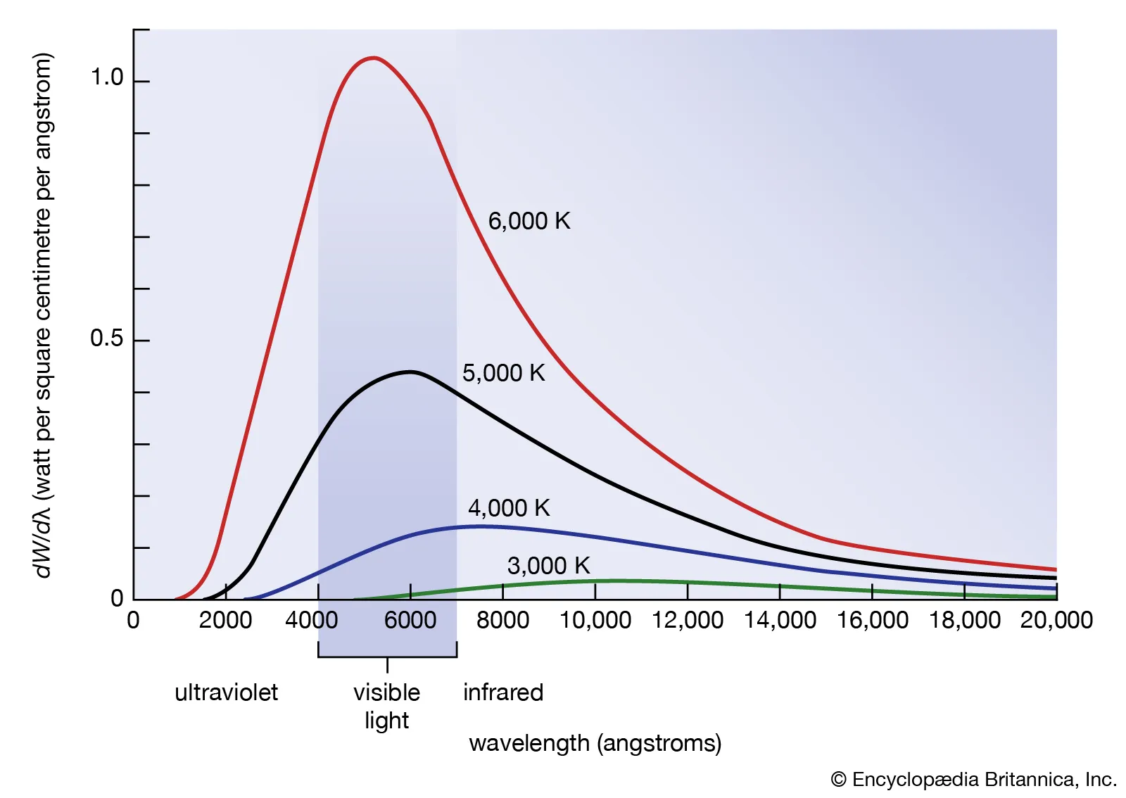
For rendering the particles into the correct primitives, there were several design choices made. Firstly, all particles were rendered as spheres with a radius specified by the physical system based on the particle mass and then scaled appropriately based on the renderer viewing angles. We utilized bidirectional scattering distribution functions (BSDF) for the spheres, but these differed for different types of particles. Particles that are actively combusting such as fuel particles above their combusting temperature threshold were modeled with an emission BSDF, since combusting fuel in an explosion should produce its own light. On the other hand, cooler particles that were not actively in combustion and soot particles were modeled with a diffuse BSDF. In both cases, the wavelengths of light emitted/reflected were estimated off of a Blackbody Radiation curve according to the particle’s temperature for RGB inputs for the primitives.

Problems tackled and lessons learned

During this process, it took a while to get the physics working, as it was a lengthy process. Since we broke down portions between multiple people, we had to communicate effectively to make sure we were all on the same page for the code. We had to decide on a baseline in order to generate an explosion, and then continue working to get the code working.

We also learned a few lessons, including that Discretized Navier-Stokes is hard! Especially in C++... Another coding lesson is to keep track of your pointers! In terms of overall project lessons, having backups for ambitious goals and modularization is important!

aaand BOOM! The Results! 💥

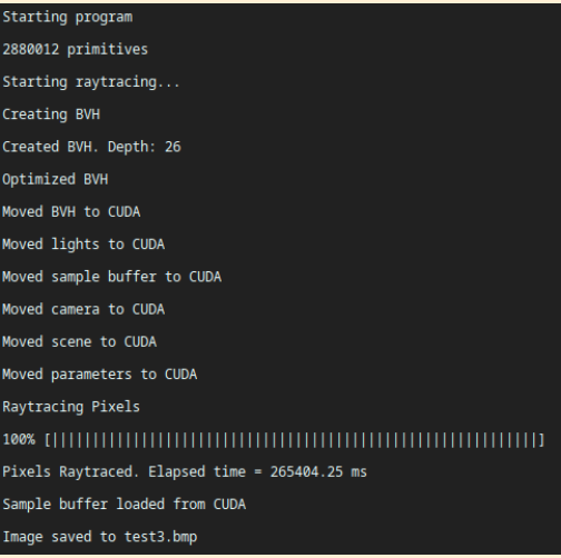
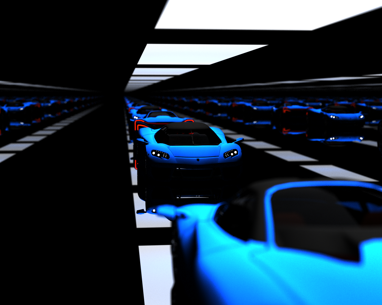
Our CUDA-accelerated raytracer was able to render the following in decent time!

Models downloaded from Morgan McGuire's Computer Graphics Archive https://casual-effects.com/data

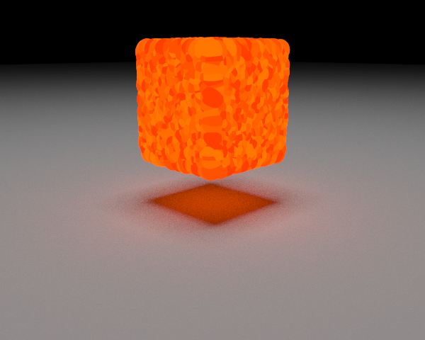
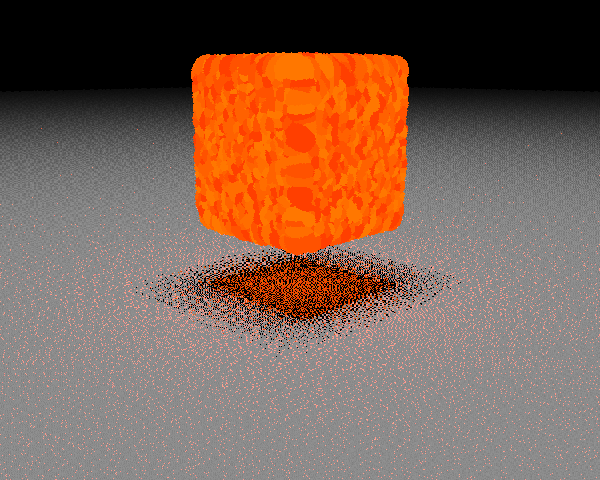
Our explosions with the fluid simulation physics:

Since Navier-Stokes is quite difficult and sometimes numerically unstable, not every rendering uses all the Navier-Stokes equations, but we managed to render some that do, which we noted! However, all of these use fluid simulation.

Below are other cool renderings that use most of the NS equations, where we varied parameters such as deviation force, acceleration due to gravity, radiative heat loss, thermal conductivity, and ambient temperature.

Before the full physical system was working, we had a midpoint animation with a basic explosion simulation, with no fluid forces:

References

https://developer.nvidia.com/blog/accelerated-ray-tracing-cuda/

http://graphics.berkeley.edu/papers/Feldman-ASP-2003-08/Feldman-ASP-2003-08.pdf

https://pages.cs.wisc.edu/~chaol/data/cs777/stam-stable_fluids.pdf

https://web.stanford.edu/class/cs237d/smoke.pdf

http://www.vendian.org/mncharity/dir3/blackbody/

https://tavianator.com/2022/ray_box_boundary.html

https://developer.nvidia.com/blog/accelerated-ray-tracing-cuda/

Contributions from each team member

Anthony: Anthony had access to the GPU and handled all of the raytracing with CUDA-acceleration optimizations on the project 3 code (module 1). Additionally, he helped with the various deliverables, and created a simplified physics model for particle only physics simulations.

Shruteek: Shru handled a lot of the physics, doing the most physics research. He set up the classes for module 2 and handled the complicated fluid physics that is modeled after Navier Stokes, and also helped with project deliverables and videos.

Srisai: Srisai handled the kinematics of the physics (forces on the particles) and also the visualizer (module 3). He worked out how to take the physics particles and convert them to primitives appropriate for the renderer, translating particle properties into primitive properties for the graphics. He also helped with the proposal and final deliverables.

Maddy: Maddy also handled the kinematics of the physics (forces on the particles) and the visualizer (module 3). She also worked out translating particle properties into primitive properties for the graphics (eg, temperature to color). She also worked a lot on the project deliverables.